HAM10000

Cancer is an ongoing health issue in our society without a significantly effective cure. It is well known that early detection of cancer may provide the patient with the best chance of beating it. Given that there are different types of cancers, each with their own symptoms, it can be difficult to detect some over others. Skin cancer is one that can be visually recognized. There are multiple different causes of skin cancer with different appearances (Actinic keratoses, basal cell carcinoma, melanoma, etc.).

In order to accurately diagnose a patient, we must take into account numerous causes of skin cancer; however, this can prove difficult as some causes can look similar at times. It may be beneficial to utilize machine learning to classify different types of skin cancers. This can help aid doctors to more accurately diagnose skin cancer by either confirming their diagnosis or suggesting a re-diagnosis. Having a second opinion from a machine learning model can help eradicate many false positives and negatives. This can ensure that patients get the most effective treatment for their type of skin cancer.

We are using the HAM10000 dataset from Kaggle, a collection of about 10k images arranged in CSV files where each column is a sequential pixel. In this section, we will detail the various models we have trained on this dataset so far.

Preprocessing  Before starting building the model, we decided to use principal component analysis (PCA) to preprocess the data due to its high dimension. We projected the points to a more manageable number of dimensions, which is ten, to de-noise the data. We used sklearn.decomposition to import PCA, which uses singular value decomposition (SVD) to project the data to a lower dimension. This will allow us to better observe and identify hidden trends and changes within the data. We intend to compare the change in accuracy between the raw data being trained on our various models (NN, CNN, Decision Tree), to the PCA-reduced data being used. Next, we created a scree plot to check whether the PCA worked well on the data or not. Based on the presence and location of an elbow in this plot, we were able to assess PCA’s performance.

Simple CNN  We constructed a simple convolutional neural net initially by using Keras’ Sequential library to progressively add layers to the network. The initial pass of the design network involved understanding the various kinds of layers that typically are used in a CNN architecture, such as Convolution, Dropout and MaxPool. One thing that we did in our initial model to greatly speed up the computation time was use batch normalization, which standardizes the input from the previous layer into a normal distribution for the next layer. This enables further activations to compute a lot faster when they receive inputs. In this first pass, the following network architecture was used: [[Conv2d -> ReLU] * 2 -> MaxPooling -> BatchNorm -> Dropout] * 2 -> [Flatten -> Dense -> Dropout] * 2 -> Dense -> Out

While we did give this model a large number of epochs to train on (75), we also implemented common techniques like ReduceLR and and EarlyStopping based on F1 score to ensure the network does not over-train. During execution, we saw the learning rate drop to extremely low values, and the network never needed to use all epochs to maximize its score.

More Complicated CNN   We used a Keras Sequential model, where each layer was added from input. We chose Conv2D, which transforms a part of an image using a kernel filter based on the given kernel size. The MaxPool2D layer acts as a downsampling filter, where it just picks maximum values within neighbors in order to minimize computational burden. Then, a dropout layer was added where some nodes are ignored (with weight of 0), making the learning process more efficient. Multiple of these were implemented in order to get a big picture of the dataset and extract several features. ReLu was used to add nonlinearity to the dataset. A flatten layer was used to make everything into 1D. The full architecture was as follows : In -> [[Conv2D->relu]*2 -> MaxPool2D -> Dropout]*3 -> Flatten -> Dense*2 -> Dropout -> Out. This particular architecture was used since it was commonly used for datasets that contained skin samples, so we used this as a starting point. The weight for melanoma was higher than others since we want the model to be more sensitive towards cancer. We used a learning rate of 0.00075 and ran it over 60 epochs with a batch size of 16 for training.

Random Forest   We decided to also look into using a random forest approach to classify the different types of skin cancer. In order to do this, we utilized the tfdf library from tensorflow_decision_forests. Additionally, we used Pandas to represent and manipulate the dataset. The program reads in the .csv representation of the dataset provided on Kaggle which includes the lesion_id, image_id, dx, dx_type, age, sex, and localization. The image_id is the name of the corresponding image (which is provided in the dataset). Dx_type, age, sex, and localization are all attributes along which splits occur in the random forest. Dx is the label corresponding to the type of skin cancer present in the image. We use a 70/30 % train/validation split. Next, we convert the labels to integers. Finally, we train the model and check the accuracy and loss graphs.

Since our dataset has 7 different types of skin cancer images, the goal of the model will be to display results as numbers 0-6, corresponding to the type of cancer the image is diagnosed as. We expect to analyze the results using methods such as accuracy and recall to test how closely our model was able to predict the type of cancer. Since there are features such as location of lesions and age included in the dataset, we hope to find out the features that impact the results the most, which would provide healthcare workers with a list of traits that make someone more susceptible to developing skin cancer. This would ideally help them warn those who are at more risk for a particular type of skin cancer based on their medical history or other factors.

Preprocessing:   The dataset was fit and transformed to create a 2D scatter plot of the features, which is shown below:

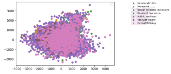
The different diagnoses are present as layers with the two features left after reducing on the x and y axes of the plot. As presented in the data, Actinic keratoses (dark purple) seem to have less correlation between the two features.

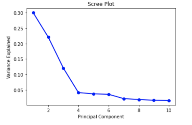
The Scree plot shown above depicts an elbow at Principal Component 4. This means that the first four Principal Components captured the most information, and the rest can be disregarded without any major loss. However, after research regarding an ideal number of Principal Components, we found that a number greater than three can imply that PCA may not be the ideal way to visualize the data. For future preprocessing, we may want to consider other techniques to reduce dimension depending on the impact of having 4 Principal Components.

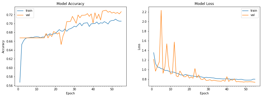
Initial CNN:  Our initial CNN used a 80/20 train-test split, and then within the training data we used another 80-20 split to extract a validation dataset. As below, we see a lot of variability in the validation dataset compared to the training set. This is likely due to the model's simplicity, which causes a tradeoff with the stability from new images. Another factor to this would likely be using BatchNormalization incorrectly, causing the normalization to happen at the wrong time. We hope to do more research on this in the next phase of the project since it is a powerful tool to speed up processing.

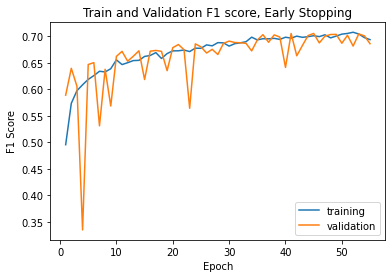
Even with varying accuracy and loss, when we plot the model's F1 score on the training and validation set, we do see stabilization as the epochs keep going.

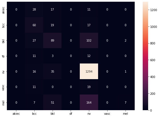
Finally, we can evaluate the model performance on the test data. The confusion matrix shows two things that we would want to improve on. First, we see no data in the akiec, vasc, and df categories, and this happened over more than one training run of the network. This could mean a bad split of test data, but is unlikely because we would have seen improvement over different runs. Thus, finding the cause of this will be paramount in the next phase of the project. The second thing we need to improve is the variability in known classifications, as seen in bcc and nv. Since we use a simple network architecture, there are likely multiple aspects of the model we can iterate on to solve both of these issues in the future.

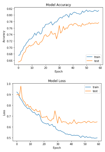
Improved CNN:   The model was evaluated using a testing and validation dataset. Loss and accuracy were used as metrics, as well as a confusion matrix. The model’s training and test accuracy and loss are shown below:

The confusion matrix for the test dataset is as follows:

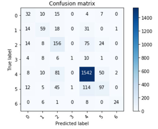
As we can see, the model does a really good job at detecting melanomas, which satisfied our goals. However, we want it to be able to classify other types just as well, so we decided to take a look at which classes were predicted incorrectly and what portion of them:

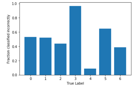
We can see that Class 3 was almost always classified incorrectly, so our next steps will also include trying to figure out why this is happening and see if we can change weights to account for this.

Random Forest:   Below are the graphs that show the accuracy and loss of the random forest on the validation data.

The accuracy graph looks pretty good and reasonable as it increases with the number of trees and seems to reach a convergence with an accuracy of around 72%. Additionally, the loss graph looks reasonable as it decreases with the number of trees. However, there are definitely measures we can take to increase the accuracy of the random forest. Below shows the architecture of the first tree of our random forest at a maximum depth of 3.

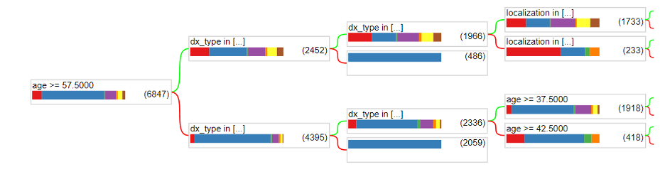
One thing to notice is that the data is not splitting by the image_id. This is most likely because the actual image was not yet used in the dataset. The only real attributes that were utilized were dx_type, age, sex, and localization. We still need to gather the pixels of each image and utilize them in a meaningful way as attributes in the random forest model. This is one way we could achieve more accurate predictions.